the remainder of the stations in the same way as you
would if the transit was set over the PC. If the setup
in the curve has been made but the next stake cannot
be set because of obstructions, the curve can be backed
in. To back in a curve, occupy the PT. Sight on the PI
and set one half of the I angle of the plates. The transit
is now oriented so that, if the PC is observed, the plates
will read zero, which is the deflection angle shown in
the notes for that station. The curve stakes can then be
set in the same order shown in the notes or in the
reverse order. Remember to use the deflection angles
and chords from the top of the column or from the
bottom of the column. Although the back-in method
has been set up as a way to avoid obstructions, it is
also very widely used as a method for laying out
curves. The method is to proceed to the approximate
midpoint of the curve by laying out the deflection
angles and chords from the PC and then laying out the
remainder of the curve from the PT. If this method is
used, any error in the curve is in the center where it is
less noticeable.
So far in our discussions, we have begun staking
out curves by setting up the transit at the PI. But what
do you do if the PI is inaccessible? This condition is
illustrated in figure 11-11. In this situation, you locate
the curve elements using the following steps:
1. As shown in figure 11-11, mark two intervisible
points A and B on the tangents so that line AB clears the
obstacle.
2. Measure angles a and b by setting up at both A
and B.
3. Measure the distance AB.
4. Compute inaccessible distance AV and BV using
the formulas given in figure 11-11.
5. Determine the tangent distance from the PI to
the PC on the basis of the degree of curve or other given
limiting factor.
6. Locate the PC at a distance T minus AV from the
point A and the PT at a distance T minus BV from point
B.
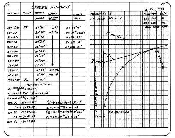
Field Notes
Figure 11-12 shows field notes for the curve we
solved and staked out above. By now you should be
Figure 11-12.—Field notes for laying out a simple curve.
11-11